ATMOSPHERIC CO2 & SURFACE TEMPERATURE
FROM THE STANCE OF A THERMODYNAMICIST;
REVISITED.
C. le Pair
clepair@casema.nl

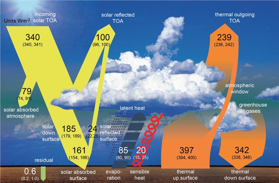
One out of several energy balance pictures. Most are based on NASA data
and adapted by various authors.
One out of several energy balance pictures. Most are based on NASA data
and adapted by various authors.
Abstract
Thermodynamics is somewhat neglected in atmospheric scientific climate considerations. Using some principles of the field sheds light on the influence of CO2 on the surface temperature. The result shows an undeniable influence, however, less than is currently assumed in IPCC reporting to decisionmakers(2).
Doubling the CO2-concentration since the year 1880 will cause a surface temperature rise between 0,56 and 1,13 °C. Presently it is about half as much.
Introduction
Since climate change became an issue, many investigations have been reported about measurements of atmospheric energy transport processes. Unfortunately their data differ somewhat. The differences lead to different expectations of even several °C about CO2-temperature relationship. A thermodynamical approach skips some of these uncertainties.
In Table 1 I list some of the data found(3).
| source* | solar absorbed
by surface W/m2 |
radiation undisturbed
up to TOA W/m2 |
latent heat
towards air W/m2 |
conducted to
convective air W/m2 |
calculated nett** radiation to
atmosphere W/m2 |
measured total nett*** radiation; (up-down) W/m2 |
|---|---|---|---|---|---|---|
| NASA-1 | 164 | 40 | 78 | 32 | 14 | 54 |
| Le Pair | 70,8 | |||||
| NASA-2 | 163 | 40,1 | 86,4 | 18,4 | 18,1 | 57,9 |
| NASA-3 | 173,4 | 20,5 | 78,2 | 23,8 | 50,9 | 51,3 |
| NASA-4 | 181 | 30 | 117 | 29 | 5 | 5 |
| NASA-5 | 161 | ?? | 85 | 20 | ?? | ?? |
| NASA-6 | 178 | 20 | 80 | 24 | 54 | 52,1 |
| Geuskens | 173,4 | 20,4 | 78,2 | 23,8 | 51 | 51 |
| Röst | 161 | 22 | 80 | 17 | 42 | 41 |
*) Data probably all from NASA, but as interpreted by different authors.
**) "atmosphere" (minus undisturbed outgoing to TOA).
***) To be compared with the sum of column 3 & 6; except in row "Röst".
The solar energy flux arriving at the top of the atmosphere TOA is about 1350 W/m2. Part of it is reflected and does not affect Earthly circumstances. A parallel beam of ~1000 W/m2 enters the atmosphere. Averaged over the surface and the year this is ~250 W/m2. For the planet to remain in a stationary state, it re-emits the same from TOA to space.
Only a part of the solar influx reaches the surface. Measurements as listed in Table 1 column 2 show a spread: 161 - 181 W/m2. The differences might be partly due to, whether it concerns only direct solar radiation or, it includes also indirect solar radiation, absorbed by the atmosphere and re-emitted to the surface. Because of this uncertainty, throughout this article calculations are done with both.
"Included" means column 2 lists the total solar input (direct +indirect), indicated as Is,t.
"not included" means column 2 lists only the direct solar input. To get
the total input, the indirect input is added separately and the total is
Is,t+. And Is,t+ = 125 + 0,5Is,t(4) .
The nett energy export from surface
In a stationary state, the surface exports the same amount of energy as it receives, either Is,t or Is,t+ , only upward. Downward transport is zero, because everything going down goes up through the same surface.
The export is by heat (conduction and convection), latent heat and by radiation.
(The radiation is not according to Stefan-Boltzmann. That law holds only for radiation to a vacuum with a radiation temperature = 0 K.)
One part of this radiation goes undisturbed by atmosphere to space. It passes through, what is called the 'atmospheric window'. The remaining part is absorbed by the air. The undisturbed radiation from surface to space has been measured. Again the reported results differ as shown in table 1 column 3.
The other exports are admitted in total to the atmosphere.
The energy flow from surface up to be handled by the air, therefore is either Is,t or Is,t+ minus column 3. To be called Ut or Ut+.
As Table 1 shows, the fluxes by conduction, convection and latent heat have been studied, again with varying results. For latent heat the range is 70,8 - 117 W/m2. For conduction and the accompanying convection the range is 17 - 32 W/m2.
Evaporation immediately stops if the air above the watery surface is saturated. This saturation is only relieved by air convection. Without, there is no latent heat transport.
The radiative part of the export, not escaping through the window, is absorbed by the air, i.e. transferred to heat to continue its outward transport through a fluid semi-transparent medium, air, i.e. also by the same convection.
Fortunately these separate contributions are unimportant. It is only the sum that counts. Air is a bad heat conductor. All heat transport through it is by convection.
The total energy export from surface till the the tropopause, except the undisturbed flow through the 'window', is done by air convection. I.e. through a semi-transparant fluid. In that stretch of path particle density is sufficiently dense to treat it with ordinary thermodynamics and mass flow dynamics.
Convective transport and CO2
From surface to tropopause the temperature gradient is conform the thermodynamic expectancy of air pressure in the Earth's gravitational field. It is only at the pause that we observe a gradually stronger deviation. The change starts at a height of 11 km as is clear from the textbook picture 1.
Picture 1
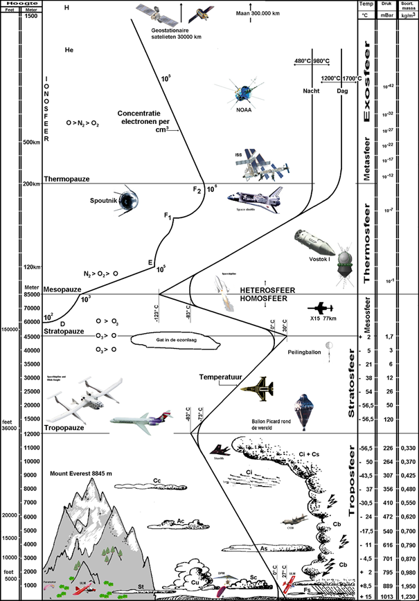 Present textbook knowledge about temperature, pressure and density against height.
The air convection length of path between surface and the onset of the tropopause is 11 km. Beyond that, radiation takes over and the dynamics mentioned is not applicable. (Above the tropopause there are even stretches where energy transport is contrary to the temperature gradient.)
The temperature at 11 km is about -55 °C (218 K). With more CO2 this does not change much. The energy flow from there to TOA remains unchanged. All that went in through the troposphere, goes out again. It is only within the 11 km thick troposphere shell that low and high resistance transport processes exchange roles.
The surface temperature at the time of most of the measurements listed was about 288 K. (And the CO2-concentration ~400 ppM. )Thus we may assume the temperature difference between surface and tropopause ∆T was 70 °C.
Heat transport in the thermodynamic media is driven by the temperature difference. This allows us to define a transport resistance R using ∆T = flow x resistance:
In this case leading to R... = 70/U.... And a specific resistance R/m = 70/11000U....
CO2 does not change the mass transport properties of air. The specific resistance R/m is invariable to CO2 up till high concentrations.
Much higher than occur in the atmosphere.
We learnt from measurements that virtually all outgoing radiation, vulnerable to CO2, is absorbed in the first 100 m of the atmosphere. If the CO2-concentration doubles (2CO2) the same absorption will take place in the first 50 m. (Not more radiation can be absorbed than emitted by the surface.) The pathlength for convective transport therefore lengthens to 11050 m. Increasing the resistance to 1,0045R for the CO2 part of the convective flow. The resistance for the other parts remains unchanged.
If the CO2 changes only from 280 ppM to 420 ppM, the same absorption takes place in the first 75 m. Increasing the pathway to 11025 m and the resistance to 1,0023R.
Absorption by CO2
We are interested in the change of ∆T by changing CO2.
More CO2 causes more absorption. But how much more? At very low concentrations - think about < 1 ppM - the absorption grows proportional tot the concentration. At higher concentrations the absorption grows slower. It is generally accepted that the reduction of IR surface radiation that passes undisturbed diminishes 'logarithmical'. It is shown in picture 2 for atmospheric conditions and surface radiation. The phenomenon(9) is referred to by several terms. One is 'spectral widening'.
With the same solar input, if less passes the window, because of more absorption, the missing part is added to the convective transport. At the TOA nothing changes. Picture 2 tells more about the phenomenon.
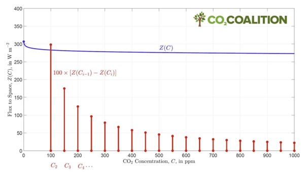
The result of 'spectral widening'; present day radiation export from
TOA vs. CO2-concentration, according to W. Happer(7).
If CO2 >> 280 ppM there is hardly more reduction of the outgoing radiation. Looking at the graph, it seems that around 400 ppM changes in the amount of absorbed W/m2 are within the range of ± 4 W/m2. Formula (1) alows us to calculate ∆∆T for different values of absorption:
First we test the results for the sensitivity to the diference of the data from different sources using formula (2), when 2 W/m2 less radiation passes through the window by CO2 absorption. This adds 2 W/m2 to Ut or to Ut+. The change in R due to lengthening of the distance to the tropopause is much smaller. Its influence will be shown below. The results of this 'source test' are listed in table 2.
| Source* | Ut | Ut+ | Rt | Rt+ | ∆∆T °C | |
|---|---|---|---|---|---|---|
| ∆Ut = 2 | ∆Ut+ = 2 | |||||
| NASA-1 | 124 | 167 | 0,56 | 0,42 | 1,13 | 0,84 |
| NASA-2 | 122,9 | 166,4 | 0,57 | 0,42 | 1,14 | 0,84 |
| NASA-3 | 152,9 | 191,2 | 0,46 | 0,37 | 0,92 | 0,73 |
| NASA-4 | 151 | 185,5 | 0,46 | 0,38 | 0,93 | 0,75 |
| NASA-6 | 158 | 194 | 0,44 | 0,36 | 0,89 | 0,72 |
| Geuskens | 153 | 191,3 | 0,46 | 0,37 | 0,92 | 0,73 |
| Röst | 139 | 183,5 | 0,50 | 0,38 | 1,01 | 0,76 |
*) Please note the reserve about NASA as source under Table 1.
When comparing the resulting temperature changes for a 2 W/m2 increase of the CO2 absorption effect, there is suprising little difference. While sources differ substantially in irradiation data minus escape through the window (123 - 158) or (166 - 194).
∆∆T may be due to warming the surface, cooling the tropopause or both. But there are more arguments not to rush to policy makers with these numbers in hand, to tell them how wrong their climate policies are.
The falacies and the merits of the presented thermodynamic approach may need more attention than in this note. For the time being I think it is remarkable that the great differences in the energy balance data gave rise to such a small variation in the final temperature results. And it highlights the importance of the outward energy transport from the surface by convection through the first 11 km of air. It is there, where the GHGs excert their influence.
This method to find a numerical CO2 - temperature relationship seems to have more advantages. It bypasses the spurious, from correlation to causation arithmetic, of Meteorological Offices World wide like the Netherlands KNMI and of IPCC report editors(5).
Another advantage is that using averaged temperatures over the Earth as a whole does not affect the energy flow, while when dealing with radiative transport, the energy flow higly dependends on the distribution of all different temperatures over the surface with their daily changes. (The Stefan-Boltzmann users falacy!)
About the human influence on the atmospheric CO2 concentration, see(6). It will take a lot of fossil fuel to double the 1880 CO2 to 560 ppM.
The NASA-1 energy balance source is used to study a wider range of CO2 absorption. The direct energy inflow to the surface from the Sun is difficult to measure. Therefore the "included" data will be used, i.e. Table 1 column 2 is the startingpoint as if it includes direct and indirect solar irradiation.
Because the resistance change due to lengthening of the distance to the tropopause has little influence, R' = 1,0023R is used. The outcomes are in Table 3.
Table 3.
| The decrease of window escape, ∆U [W/m2] effect on ∆∆T [°C] | ||||||
|---|---|---|---|---|---|---|
| -10 | -8 | -6 | -4 | -2 | -1 | 0 |
| -5,65 | -4,52 | 3,39 | -2,26 | -1,13 | -0,56 | 0,00 |
| 0 | 1 | 2 | 4 | 6 | 8 | 10 |
| 0,00 | 0,56 | 1,13 | 2,26 | |||
Cooling and warming by less and more CO2.
At ∆U = +4 and path length 110025 m, R' =1,0023R ∆∆T = 2,43 [°C]
Table 3 does not show a logarithmic deminishing change with rising ∆U. Well, tables are for numbers, not for graphic expression. That becomes clear, when keeping in mind, and looking at Happer's graph, that ∆U = 0 corresponds with 400 ppM, ∆U = 1 W/m2 ↔ 470 ppM and ∆U = 2 ↔ ~560 ppM. Beyond ∆U = +4 is even unthinkable. There is not enough fossil fuel for it.
With lessening absorption ∆U = -10 ↔ ~80 ppM. That is way accross the limit, where plant life and our life on Earth are impossible. A warning against plans to suck CO2 from the atmosphere and storing it irritrievely.
As was said before, lengthening of path from surface to tropopause by CO,2 is negligeable. The change from 2,26 °C to 2,43 °C is irrelevant in view of the data spread.
Conclusions
These notepad calculations about thermodynamic and fluid dynamic processes related to the energy balance and the temperature distribution of the Earth, show their relevance for climate. It is worthwhile to refine them, if more certainty of the relevant data would become available. They obviously don't support the hypothesis, that the Earth is in an emergency situation because of fossil fuel use.
Perhaps the most important is, they justify a definit stop to the reliance in the fear mongering results of present day climate models.
Acknowledgement
A note with the used data and the main characteristics of this article circulated among a group of colleagues. I am grateful to W. Happer, A. Huijser, W. Röst, C.A. de Lange for their interest, their comments and critics. They supplied additions to the database and encouraged me to publish a revised version, To find out what a wider group of readers think about it.
Nieuwegein, 2023 09 11.
Revised version, 2023 09 21.
Notes & References
- C. (Kees) le Pair, PhD Physics and Technology, Leiden & Delft, ex director of The Netherlands National Research Organisations for these two disciplines FOM and STW. In a previous article the thermodynamic approach was mentioned and probable results indicated.
- SR1.5: Global Warming of 1.5°C "The likely range of total human-caused global surface temperature increase from 1850-1900 to 2010-20197 is 0.8 °C to 1.30 °C, with a best estimate of 1.07-0.8 °C. Over this period, it is likely that well-mixed greenhouse gases (GHGs) contributed a warming of 1.0°C to 2.0 °C , and other human drivers (principally aerosols) contributed a cooling of 0.0°C to 0.8 °C, natural (solar and volcanic) drivers changed global surface temperature by -0.1 °C to +0.1 °C, and internal variability changed it by -0.2 °C to +0.2 °C."
- The table contains data attributed to NASA. It is not certain that authors did not adjust them according to their own interpretations. Honor to Kiehl & Trenberths, whose early results were used in IPCC's 3d report in 2001.
- When table 1 column 2 represents only the direct input from the Sun, this means that 250 - column 2 or (250 - Is,t) has been absorbed by the atmosphere. The air exports it arbitrarily up and down, either as radiation or heat. However, in the low troposphere the temperature gradient impedes downward transport of heat. Thus the indirect downward energy import is < 0,5(250 - Is,t). The surface receives in total somewhat less than 125 + 0,5Is,t. Mind, the uncertainty is halved.
- The use of CO2-concentration relation with temperature to derive a causal dependence is invalid. The statistician Yule showed this already in 1926. He called it 'spurious correlation' of two monotonous rising data series.
- A. Huijser & C. le Pair: How does our CO2 escape?
- W. Happer calculated the undisturbed outgoing IR from the surface using MODTRAN. Above 280 ppM more CO2 changes little.
- C. le Pair: The GEO triad of the Earth's greenhouse.
- J.M.J. van Leeuwen, priv.com., argued that the logarithmic description of the process should probably be based on a Lorentzian. This because the molecular collisions disturb the normal energy levels of the molecules. He referred to W.J. Witteman: "Global warming by thermal absorption of CO2" on this site or on Principia Scientific.
| → top | → index |
|---|