

by
C. le Pair & A. Huijser
correspondence: clepair@casema.nl
A popular version (in Dutch)
CO2-groei.
can be read on Climategate.
Abstract
The increase of CO2 into the atmosphere due to fossil fuel is exceeding the measured accumulation. A part of this excess CO2 is dissipating into the ocean and other CO2-sinks. The dissipation rate can be derived from reliable data. The CO2 flows are modeled using a physics decay formula, which fits the data between 1880 and 2020. It is robust enough to use for extrapolation in scenarios of future increase of atmospheric CO2 due to fossil fuels. It is determined that the half life of the remaining excess CO2 is ~37 year. If the use of fossil fuel would stabilize at the level of years 2019-2020, the atmosphere would contain ~515 ppM in the year 2100.
Doubling, however, is beyond scope. If the increase of fossil fuel use would persist at a rate of 1,5%/yr, we should expect 647 ppM in 2080.
The assumption is valid, that excess CO2 is caused by the use of fossil fuels. However, the increase would be limited also in its consequences.
Content
1. Introduction
Carbon (C) is a vital element. Plants and animals are built with molecules containing C. Plants on ground and in the ocean feed on atmospheric or dissolved CO2. Animals derive their carbon directly or indirectly from plants. Without CO2 no life, as we know it, would exist.
In 2020 the concentration of CO2 molecules in the atmosphere is ~415 ppM. (415 CO2 molecules in one million molecules of air.) 20.000 years ago, at the end of the last glacial it was 180 ppM. Dangerously low, because with less than 150 ppM plants on land will not grow.
On the other hand a few percent of CO2 in the air would suffocate us. During the last 150 million years the atmospheric concentration declined from ~2000 ppM (0,2 %) to 0,04 % at present.
We are living in a period with ample higher and lower safety margins. Still there is commotion about atmospheric CO2. Currently the contents increases ~2,4 ppM/yr, according to measurements at many places around the globe notably at Mauna Loa Observatory (MLO or ML for short), on the island of Hawaii in the
Pacific. The ML measurements are generally considered representative for the atmosphere as a whole, due to winds stirring the air. NASA Goddard's Space Centre composed an interesting animation of the mixing process based on its satellite measurements(1). The variation around ML's average data is ±10 ppM, rapidly changing locally.
There are many C-storages. Trees, books, furniture, houses, ships, plants, shells, rocks, whole mountain ranges, peat, coal, oil, gas, the ground below land and sea etc. These contain much more C than the atmosphere. And they are in constant exchange with it; some in slow, some in fast processes. Erosion of limestone rock and outgassing is a process lasting hundreds of millions of years like the storage of CO2 by Olivine, the world's most abundant mineral. Corals are building islands of calcite skeletons within a couple of years. Flying insects supply the atmosphere with ten times more CO2 than mankind with all its machines. They consume herbs making room for new growth, that absorbs CO2 from the atmosphere Here we deal with cycling times from days to a few years. For trees it may take many decades before they die and decay, or are burned in wild fires or by us. Volcanoes and such fires deliver sudden big CO2-surges at irregular intervals...
Storage and transport of carbon reserves have been investigated abundantly. F. Engelbeen(2) reviewed and elaborated on several processes with special impact on the atmosphere, referring to earlier work by others. We apologise for not doing that again.
A special case for carbon storage and transport is the oceans. These contain 50 - 100 times more CO2 than the atmosphere. What happens depends on the storing mechanism. There is solution in water and, depending on salinity, also dissociation and chemical storage. Each with their own typical intake and out flow process times. In chemical equilibrium with pure water CO2 behaves like inert gasses. It follows Henry's law. In the low concentration range, we are dealing with, this would hold also for other storing mechanisms in sea water. The solubility would be proportional to the partial CO2 pressure in the gas phase. So the ocean would capture 98% of any quantity added to the atmosphere and the fossil contribution would be insufficient to explain the ML measurements.
Solubility depends on temperature. It decreases when the temperature rises. This effect explains a rise in atmospheric CO2 of ~100 ppM between the ice age and the present interglacial. One of us checked whether the rising temperature between 1880 and 2020 could be the cause of the present increase(3). It isn't13. The temperature change would make up for some 12 ppM rise instead of ~120!
Much depends on the time it takes to reach equilibrium between the atmosphere and other CO2 stores. If relaxation times would be in the order of one or two years, the origin of CO2 excess would be a puzzle. With the IPCC assumption of 100+ years, we would end up with catastrophic forecasts, from a climate point of view.
The commotion around atmospheric CO2 is not about starving plants or suffocating animals. One assumes that more CO2 increases the Earth's temperature. It melts land ice and expands the water volume. The sea level rises and low lying lands will be flooded. There are more consequences, both annoying and favourable. Enough to justify an investigation. However, when studying the available data, we discovered, it is not so much a matter of "where does all this CO2 come from?" But rather, "how does all that CO2 disappear?"
2. Process times
Figure 1
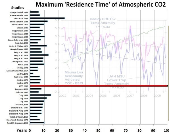
Several researchers attempted to find the residence time for atmospheric CO2 relative to many other CO2 stores. Others made compilations thereof. The results range between 2 - 28 year. The IPCC's "Bern model" stands out with its 100+ year. Figure 1 pictures the harvest of results. It is only to show the lack of consensus as different definitions of process times were used.
Atomic atmospheric bomb tests provided researchers with a carbon tracer. This enabled them to calculate the process time of atmospheric refreshment. Each year about 1/7th of the atmospheric CO2 is exchanged with numerous sinks and sources. So, at first sight, one would expect a half life of refreshment of about 10 year. And that is what, according to several authors, this tracer study showed. Refreshment, however is different from a process of reaching equilibrium after a pressure or concentration excess. Refreshment occurs independently of excess pressure or concentration. The refresh exchange between atmosphere and other sinks is limited to a rather thin boundary layer or a small in-and-out taker, whereas the store of CO2 is within the whole bulk. In many media the internal mixing or transport of CO2 is much slower than in the atmosphere.
Disregarding this difference caused much confusion about decay time of added CO2 as well as the cause of rising atmospheric content.
The previous article(4), in which one of us tried to answer the question "How does all that CO2 disappear?", was based on sloppy, noisy data. Results from scattering data depend strongly on the way of averaging. It is only during the last fifty years or so, that the 'signal' exceeds the noise, i.e. the natural fluctuations. Hence, here we used the best 'state of the art' available data, and we changed the computation from the integral to the differential processing. This also offers a wider range for conclusions about related consequences.
The presumption is simple. The atmosphere is a reservoir. It accumulates by many sources and dissipates CO2 into many sinks. We know how much fossil CO2 we put into it. And we measure that its increase is less than the fossil fuel supplies. So for many years all the other sources and sinks together act as a net joint sink. We check whether an accepted physics theory describes this joint behaviour.
Others did the same, as we learned from comments we received after appearance of the earlier article(2,5). Roy Spencer(6) and Peter Dietze(7) recently used a similar approach as we did. The results are mutually confirming within the margins of scattered data they used.
3. Data and method
-
Reliable data we used are
- ML annual average CO2 concentrations (ppM) 1960 - 2019.
- CDIAC (US Dep. of Energy DOE) (https://cdiac.ess-dive.lbl.gov/). Amount of fossil fuel tons of oil equivalent (toe).
- Conversion of atmospheric 1 ppM CO2 = 2,12 GtC = 7,77 GtCO2 (GtCO2 = 1000 million ton of CO2). Following CDIAC, IPCC a.o..
- Data and the algorithms we used can be found and downloaded in the Excel spreadsheet
The CO2 concentration in the atmosphere at time t is N(t). It changes due to many sources and sinks. One of them is the annual anthropogenic fossil CO2 supply B(t), which is fairly well known. We are interested in the behaviour of all other sources and sinks together. Looking at ML annual increment data from 1960 onward, and comparing with the fossil CO2 input, it is obvious that CO2 disappeared. All other sources and sinks together act as a fluctuating but on the average, steadily growing sink. If the system would be in equilibrium, there should be equilibrium concentrations in all subsystems. We assume such an equilibrium existed at some time t = 0. The atmospheric concentration at the time being N(0). In nature there are many such systems in which equilibrium conditions are approached at a rate proportional to a driving force. In this case that would be the concentration difference between N(t) and N(0)(9). This leads to a differential equation
Herein the constant proportionality factor is 1/T. T is the characteristic residence time of excess CO2 in the atmosphere. (In the previous article(4) the integrated formula was used with k as flow coefficient; k = 1/T.)
Even when the other sinks and sources would also change with a rate proportional to N(t) - N(0) but at a different Ti, formula (1) still holds with
1/T = ∑ 1/T i. This approach even holds for slow changing conditions in the various processes like e.g. the pH balance of the oceans, which will shift the equilibrium concentration for that CO2 absorption process. The same happens with variation in temperature.
Irregular CO2 sources like volcanism, extreme wildfires or influences from phenomena like El Nino/La Nina in the past are part of the Mauna Loa data. They seem to have had virtually no impact on the trend. That is fortunate, because when in future some unforeseen big event happens and we know how much CO2 it involves, we shall be able to predict from that moment on, how N(t) will evolve further. That is, if T and N(0) are firmly established.
Another - fortunately unlikely - disturbing factor would be the appearance of an unexpected new trend source or sink. We don't know, what we know not.
Please note. This paper focusses on long-term trends and will only use eq. (1) averaged over the annual cycle to take out any season related effects that are otherwise very well visible in atmospheric CO2 monitoring data.
Furthermore, eq. (1) is a specific form of the general relation between the rate of change of the atmospheric concentration N(t) and the sum of all sources Bi(t) and sinks Si(t)
dN(t)/dt = ∑ (Bi(t) - Si(t)) (2)
It is tempting to take into account all individual sources and sinks. This is, what e.g. the Carbon Project does(8). Next to the fossil fuel emission source B(t) in eq.(1), the project provides best guesses about all other contributing processes like for instance deforestation, change of land use, degassing of rock etc.. It also considers the various sinks like the ocean, soils and biosphere with their specific parameters for these different CO2 absorption processes. Recently this was extensively reported by P.Friedlingstein & some 70+ colleagues(8).
However, we only use their data of fossil CO2 supply as
we are on a different track. Our aim is to single out the role of fossil CO2 'vis à vis' the other sources and sinks together. We wanted to see if the data, we consider reliable, show some joint behavior, allowing to calculate from eq. (1) stable values for T and N(0). Otherwise we cannot use these thus obtained values again with eq. (1) in forecasting the development of CO2 concentration in the atmosphere depending on various fossil fuel consumption scenarios.
The data listed and computed in the Excel sheet to be downloaded are depicted in figure 2.
Figure 2
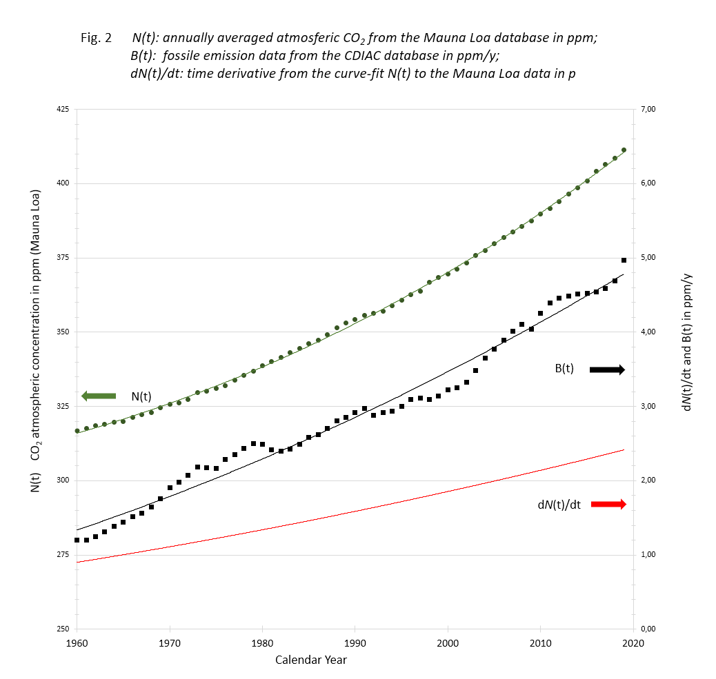
N(t): Data of Mauna Loa annual CO2 averages with accompanying 3rd degree trend line;
B(t): Data of Carbon Project fossil fuel and cement emissions with 2nd degree trend line;
dN(t)/dt: time derivative of the N(t) trend line.
The Mauna Loa data show a smooth monotone increase over the years, although the yearly increments scatter. The carbon data are annual contributions fluctuating because of fluctuating human activities.
In order to test the stability of the decay time, we computed T for three different equilibrium concentrations N(0): 280, 287 & 294 ppM, using the rewritten formula (1):
The results are shown in figure 3
Figure 3
3.png)
Variance of decay time T over the years with different assumed equilibrium concentrations.
Although indicative, the outcome of this analytical approach with curve-fitted polynomials for determining N(0) and T is not sufficient as the variations in T over the years seems to be too big to justify
the method. But then we should realize that the approach
uses the data with equal weight and that due to the long residence time we apparently have to deal with, small errors in the early years of this period have a far to "heavy" weight in the overall outcome. Using these results for forecasting of the effect of future emission scenarios would therefore lead to questionable results.
4. Optimizing T & N(0)
To obtain more accurate and stable results, we apply eq. (1) to reconstruct the development of the atmospheric concentration from 1960 to 2020 purely on basis of the original fossil fuel emission data. For that purpose, we rewrite eq. (1) into a recurrent relation between the CO2 concentration C(t) in any year to the concentration a year earlier plus the fossil emission B(t-1) in that year minus the amount of CO2 that has been absorbed in the sinks of the environment, i.e. {C(t-1)-N(0)}/T:
It is obvious that for this reconstruction we need input values for Ni(0) and Tj as well as a value for the concentration at the starting point from which we will build up this C(t) sequence.
By comparing the thus obtained sequence C(t), Ni(0) and Tj with the measured data N(t) for every year, we can apply a straightforward "minimum average least square" approach in an iterative process to determine the optimum N(0) and T values.
Those values also depend on the starting point we have chosen to build up that particular sequence. Although it seems logical to take the concentration in the year 1960, N(t=1960) and build the sequence C(t) from there on, there is no guarantee that any particular starting concentration isn't biased by a non-predictable emission-event as discussed earlier in the introduction. Such a bias would propagate through eq. (4) and heavily influence the end-result like in the analytical approach. So, as any choice for a starting point would be subject to such an unknown bias, we should do in principle this optimization process for all starting points in this period 1960 to 2019 and take an average of thus obtained ensemble of 60 different N(0) and T combinations. Realizing the amount of work we started with the most simple approach of taking the two most extreme starting concentrations N(1959)and N(2019) respectively, and reconstructed their corresponding time sequences of "up" and "down" concentrations C(t), took the average of both and determined N(0) and T as described. We checked this approach by applying a more extensive calculation using 7 different starting points 1959, 1969, 1979,..., 2019, but found no significantly different N(0) and T values as from the "2-way reconstruction".
Figure 4a shows the outcome of this exercise, in the form of the standard deviation σ between these sequences for a 3x3 set of N(0) and T values, centered around their optimum values. We have chosen the values of this matrix in such a way that the non-centric combinations show at least a value of 2σ, indicating a rather steep minimum of the "sum of squares" surface in the [N(0),T] space.
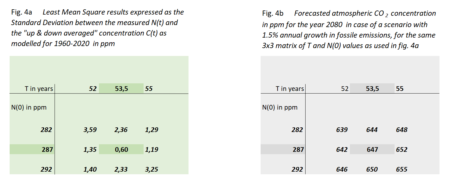
Through this we arrive at the most reliable values of N(0) & T:
Decay time T = 53,5 year (equal to half life th = 37 year)
In figure 4b we show to which value of C(T) these 9 cases would lead in the year 2080 if fossil fuel use keeps growing with 1,5%/yr. The most likely result is 647 ppM in 2080 with a limited spread of less than 1%.
We speculated on the 7 ppM difference between the most quoted 1880 CO2 concentration (280 ppM) and the one found this way (287 ppM). In a previous paper(3) we looked at the change in equilibrium partial pressure with changing temperature(10). In pure water the change would be about 12 ppM/°C, while for the salty oceans we have seen some 16 ppM/°C. The latter thanks to differences between glacial and interglacial.
One is tempted to ascribe the 7 ppM difference to the matrix iteration result to half way between 1880 and present temperature of the oceans.
5. Results
The proof of the pudding... In order to check the decay theory, we plotted the calculated C(t) using measured B(t) against the measured N(t) of Mauna Loa. We used the optimized values of T and N(0). See figure 5.
Figure 5
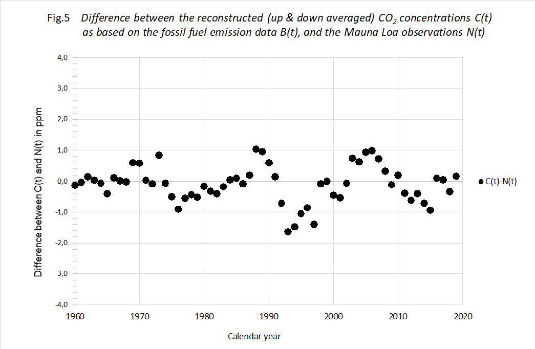 We think there is a striking result. The theory allows for a prediction of the Moana Loa measurements within ± 1,2 ppM virtually over the entire 60 year period. This difference between reconstructed and measured data is extremely small, also in the early years of the period. Add this to the knowledge that back from 1960 the increments in fossil CO2 are further declining, making the fossil CO2 influence less and less, we feel pretty confident that our formula (1) describes the
atmospheric CO2 concentration over the entire industrial period of about 140 years with an accuracy within ± 0,5%. Or rather it describes the CO2 loss each year with appreciable precision.
We think there is a striking result. The theory allows for a prediction of the Moana Loa measurements within ± 1,2 ppM virtually over the entire 60 year period. This difference between reconstructed and measured data is extremely small, also in the early years of the period. Add this to the knowledge that back from 1960 the increments in fossil CO2 are further declining, making the fossil CO2 influence less and less, we feel pretty confident that our formula (1) describes the
atmospheric CO2 concentration over the entire industrial period of about 140 years with an accuracy within ± 0,5%. Or rather it describes the CO2 loss each year with appreciable precision.
Although it goes beyond the scope of this paper, the pattern of
variations between calculated and measured data can probably be linked to certain events like volcanic activity or large wildfires, that had major (order of 1 ppM) impact on the CO2 concentration.
Another test for the model is the comparison between the fraction of B(t) each year that stays in the air, the 'airbound part', and that fraction according to our calculations. It is shown in figure 6
.
Figure 6.
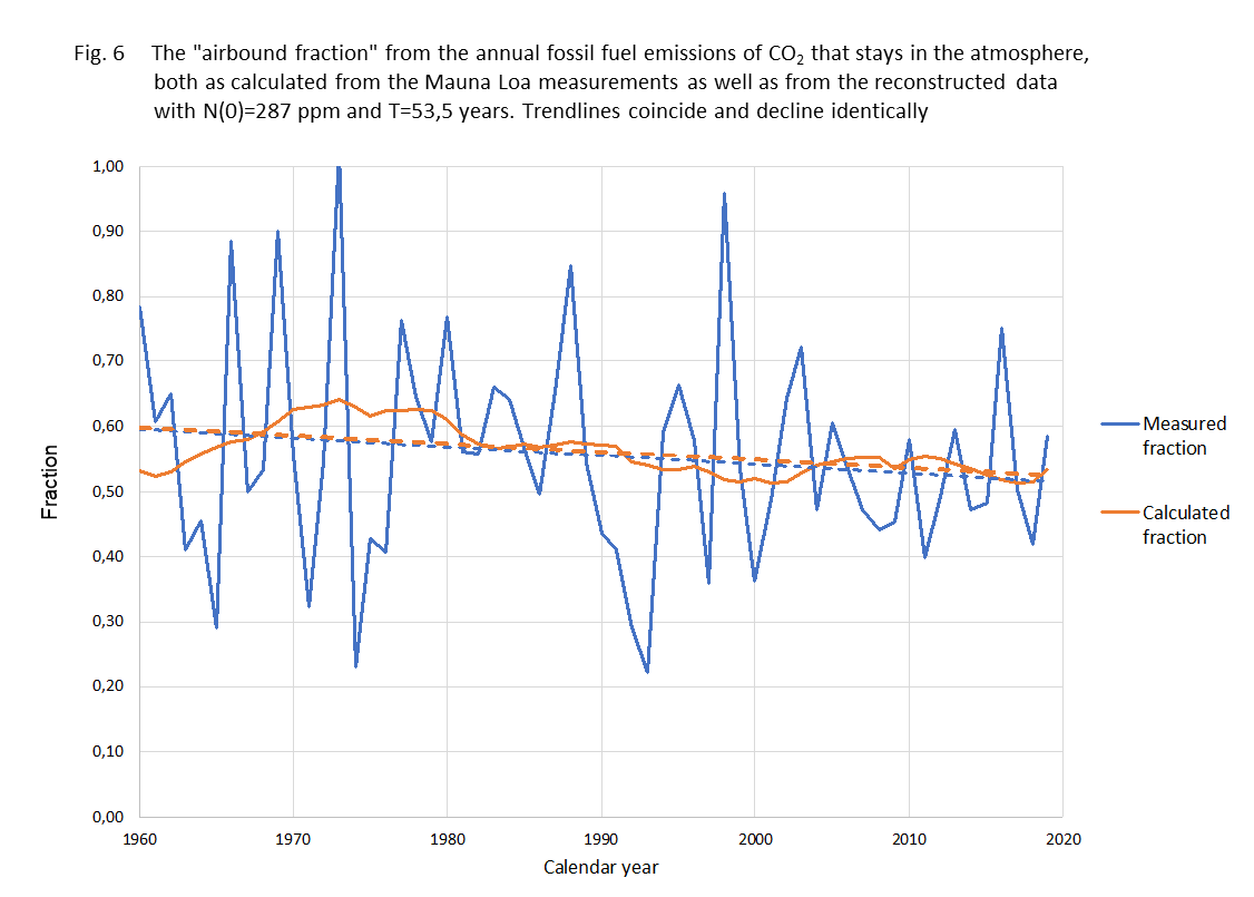 Fraction of annual fossil added CO2 that stays in the air the same year.
blue line - measured data
yellow line - calculated rresult
blue dashed -linear trend measured...
yellow dashed - linear trend calculated result
The method shows to be sturdy against different kinds of averaging. The trend from the data and from the calculations are virtually the same. It might be good to mention here that the "airborne fraction" is just an outcome of a comparison between actual CO2 concentration and the increase over the last year. It is certainly not the fraction of anthropogenic CO2 that remains in the atmosphere as some "climate alarmists" suggest. As the natural CO2 emission and absorption streams are much larger than the anthropogenic contribution, most of the excess will therefore be from natural origin and most of the anthropogenic CO2 even absorbed. As CO2 molecules aren't "labeled" (we do not engage in any discussion about the isotopic fractions) we just describe the "net"-effect.
This accuracy is again an implicit validation of the simple model of eq. (1) for the way the earth system reacts to CO2 emissions of non-equilibrium nature. And with that observation we dare to use it as a simple tool to forecast future developments in relation to scenarios for the anthropogenic emission in the years to come.
To do so, we applied eq. (4) to four different scenarios for the release of fossil CO2 into the atmosphere each year.
- N(t) 'business as usual' growth of fossil CO2 emissions 1,5 %/yr.
- N(t) with the same fossil emission as present, i.e. 5 ppM/yr.
- N(t) as II but now with a reduction of 1,5% annually.
- N(t) for immediate ban on all fossil fuel use.
The result of the exercise is depicted in figure 7, drawn lines. We added a tail of the historical process. There, on this scale, is no difference to be seen between the actual data and the computed results.
Figure.7
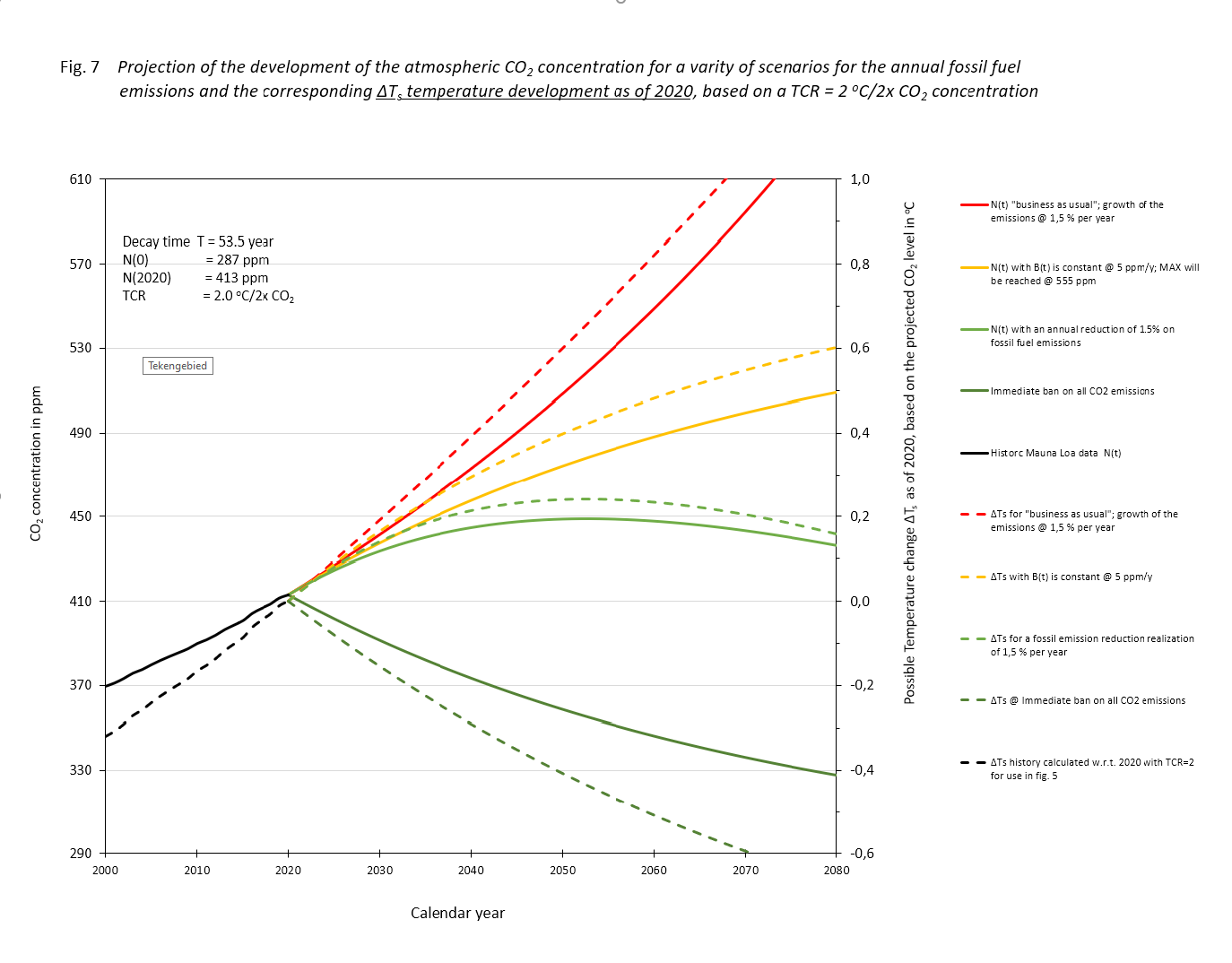
If the fossil CO2 emissions in the following years remain as present, scenario (II), we 'll see a rise until we approach a level where the natural sink approaches the input of 5 ppM/yr at 552 ppM. It won't rise above that level, which is less than two times the equilibrium of 287 ppM. That 2x the pre-industrial level will never be reached.
With a mall annual reduction of -1,5 %/yr, (scenario (III), the maximum will be reached around the year 2050 at a level of about 445 ppM. After that there will be a lowering, first accelerating and then slowing when approaching 287 ppM.
In scenario (I), the exponential growth case of fossil fuel use, 1,5%/yr, the atmospheric concentration will be double the equilibrium value before the year 2070. The growth will continue till all fossil fuel is depleted.
6. Side step for policy makers
In fig. 7 we have shown graphically the development of the atmospheric CO2 concentration for a number of future fossil fuel emission scenarios using the recurrent expression of eq. (4). All these scenarios that can be more generally described as B(t) = B(0). e(a.t) )(a being a reciprocal time constant, with a = 0 for the case B = constant) can also be solved analytically using eq. (1). However, policy makers are not as much interested in the development of the CO2 concentration for certain scenarios as such, but more in the maximum value it will eventually reach. In case there is indeed for a certain scenario a maximum CO2 concentration Nmax, this value can be easily expressed by using eq. (1) under the condition dN(t)/dt = 0:
which can only be true if the development of B(t) levels off at a certain time at a maximum of Bmax.
The determination of N(0) and T in this paper makes the expression in eq. 5 powerful, as it quantifies the effect of measures on fossil fuel emission for the expected atmospheric CO2 concentration. With current assumptions in climatology (AGW hypothesis), this is a determining factor for the change in the Earth's temperature. Although the importance of CO2 for the temperature is contested, it might be interesting for policy making to quantify the consequence of our findings in case they think the AGW-hypothesis is right.
If so, eq. (5) can simply be used to calculate the maximum temperature increase in relation to Bmax by applying the climate
sensitivity expressed as the Transient Climate Response, TCR i.e.
the temperature change in degrees centigrade when the CO2 concentration
doubles:
If we would take the Paris agreement of a maximum acceptable temperature raise relative to pre-industrial conditions of 2 degrees centigrade, and a TCR of 2, eq. (6) leads directly to a Bmax = N(0)/T. With the values for N(0) = 287 ppM and T = 53,5 years, Bmax = 5,4 ppM, about the current level of fossil fuel emissions annually. For the four scenarios depicted in fig. 6 we have also added the corresponding temperature developments (dashed lines) applying a TCR = 2℃/2CO2. Mind that the temperature developments as shown in fig. 7 are calculated according to ΔTemp = TCR.ln(C(t)/N(2020))/ln 2, i.e. relative to the temperature in 2020 and not relative to the pre-industrial level. The idea of some, that we have to go back to temperatures in those days is not realistic, if not even completely wrong for our wellbeing.
We are well aware that the outcome of the possible temperature increase as calculated by applying eq. (6) depends not only on the values for N(0) and T which are determined in this study, but depends as much on the choice of the value for the TCR, or even more fundamentally, on the choice of applying TCR or ECS, the Equilibrium Climate Sensitivity. Both TCR and ECS concepts are still subject to many debates in which we don't want to get involved.
We only want to illustrate how our findings on the development of atmospheric CO2 concentration, can be "translated" in a pragmatic way. Thus providing policy makers who want to follow the AGW-hypothesis and plan to take measures to limit CO2 emissions accordingly, with simple and transparent models. At present, all policy making is based on the output of very complex Global Circulation Models (GCM's); calculations that nobody outside the small, inner circle of climate experts can verify. Eq.(5) and (6) provide such a simple model and people are free to put in their own "beliefs" regarding the climate sensitivity to CO2 levels. Our choice for TCR = 2 is just to illustrate the strength of eq. (5) and (6).
A recent study of Schurer et al(12) based on a thorough analysis of existing temperature data yields an estimate TCR = 1,7 ℃/2CO2 within a 90% certainty range of 1,2-2,4. While Witteman(11), using a 'first principles' method of assessing the CO2-temperature relation, concluded 1/10th of the IPCC assumption. Which means TCR ≈ 0,2 ℃/2CO2.
7. Conclusions
In the preceding paragraphs we have included our comments about the precision of our computation and the data we used.
This article supports the statement
This holds for the period 1960 - 2020 and most likely even 1880 - 2020. In this period all other sources and sinks together have acted as a steady sink for atmospheric CO2.
The joint sink acts at a rate proportional to the difference between
actual partial pressure and equilibrium partial pressure.
of fossil fuel use persists through the next century.
For that scenario to continue there is not enough fossil fuel.
Whether all of this above is just merely a data fit, or a real theory of the system? Only future can tell.
This article together with its attached Excel sheet to be downloaded, provides a tool for future tests of currently circulating climate model studies.
2020 06 08
8. Acknowledgment & additional comment
We gratefully acknowledge the following colleagues for valuable comments, criticism and help; André Bijkerk, Wim Witteman, Ferdinand Engelbeen, Frans Schrijver, Peter Dietze, Chris Schoneveld, Guus Berkhout, Brendan Godwin.
We did not include all remarks we received and all remaining flaws are entirely the responsibility of the authors.
Additional: P. Dietze(7) found th = 38 yr, almost the same as we did ( th = 37 yr ). He also extrapolated this for a scenario with constant fossil input. However he introduced a fast 33% enlarged buffer to cope with "light biomass, surface water and soil moisture". That led him to predict a maximum atmospheric concentration of 487 ppM, while we calculated a maximum of 555 ppM in that scenario without an extra buffer.
Revisions 2020 07 14,
2021 06 20,
2021 06 06 & 2022 08 23.
9. Notes
Our data allowed for computation of a more likely equilibrium concentration of 287 ppM.