This article is posted
for review. The author
welcomes comments.
Electricity in The Netherlandsa.
Wind turbines increase fossil fuel consumption & CO2 emission.
C. le Pair
clepair@casema.nl
Abstract
First we describe the models presently used by others to calculate fuel saving
and reduction of CO2 emission through wind
developments.
These models are incomplete. Neglected factors diminish the calculated savings.
Using wind data from a normal windy day in
the Netherlands it will be shown that wind developments of various sizes cause extra fuel
consumption instead of fuel saving, when compared to electricity production with modern
high-efficiency gas turbines only.
We demonstrate that such losses occur.
Factors taken into account are: low thermal efficiency at low power; cycling of back up generators;
energy needed to build and to install wind turbines;
energy needed for cabling and net adaptation; increase of fuel consumption through partial replacement
of efficient generators by low-efficiency, fast reacting OCGTs.
1. Introduction
Several countries are investing heavily in the construction of wind turbines
reportedly to save fossil fuel
and to reduce CO2 emission. The wind comes free,
the turbines do not pollute and there is no need to burn fossil fuel. However, this simple notion
defended by staunch supporters of windturbines, has been criticized by several critical analysts,
e.g. refs: 4, 5, 6, 8, 10, 11, 12.
Wind does not blow according to the demand of electricity users. Sometimes there is no wind or
too little
wind, or too much. It would be no problem if there was an economic and practical way to store
electricity and to use it from that storage whenever needed. Unfortunately we
currently do not have such
a storage option. Batteries have little capacity and they are much too expensive. There are other
possibilities but none of them comes near to anything that is economically feasible. There is hydro power,
(i.e. lakes in mountains) that can be pumped full if there is an electricity
surplus and emptied when the power is needed. But this adds more cost to an already high-cost option.
(With hydro storage, one loses a quarter to one third of the energy input.) For geographic reasons, most wind development
locations don’t have this option anyway. This is certainly the case in the Netherlands.
So the current practice is to have wind developments operate in connection to conventional powerplants.
These generators step in when the wind fails and they can be switched off, or their output is reduced,
if the wind blows. Thus, when considering wind power, one must factor
in an augmenting conventional system (typically gas).
A handicap complicating the selection of options is the absence in the public domain of
factual data about the different producing units. So the arguments are mostly based on model computations, but
there are exceptions. In the USA a BENTEK study
used real emission data of power plants in Texas and Colorado. They became available due to
the Freedom of Information Act. Its conclusion was: wind has no visible influence on fuel
consumption for electricity production and the emission of CO2
in the atmosphere is not reduced13.
This shocking result did not convince decision makers yet. The negative result
was attributed to a difference in fuel mix. Coal-, oil-, gas- and nuclear heated generators
behave differently. So what might be true in that study, does not mean that it holds true for all of us.
In August 2011 Fred Udo analyzed the data put on the internet by EirGrid, the grid operator in Ireland. His web page article was termed by colleagues abroad 'The smoking gun of the windmill fraud'. He showed that a substantial wind contribution in the Irish Republic caused such a small saving of fuel (and of CO2 emissions), that it shattered a major tenet of the wind policy. He also was able to show that more wind penetration caused an increase of CO2 emission8.
The real situation, however, is even worse. The way EirGrid derives its data on
CO2 emission does not correlate with what is actually happening
in fossil fuel power plants. Moreover the Irish data does not include some other
serious factors that further undermine the
desired fuel savings. There is evidence that
the overall CO2 emission in Ireland can be ~20% higher
than the emission calculated in the EirGrid tables, as Udo showed.
(His source: ref. 14. A difference of 3% might be due to the importing
of electricity. Transport losses have been accounted for.)
We believe even Udo's figures to be conservative. On
the basis of existing data plus new information on the behavior of conventional generators when
they are cycling (i.e. ramping up and down in order to compensate for the variations in wind power) we
shall show how much worse the influence of adding wind electricity to the grid really is.
2. The old model.
During the early days of modern wind turbines the academic argument was simple and appealing:
every
kWh electric energy generated by wind replaces a kWh produced by a fossil fueled power plant.
As a result supposedly diminishing fossil fuels are saved and the CO2
that would be produced is not released in the earth's atmosphere.
Different generators have different thermal efficiencies, and the CO2
production is different for gas, coal and other fuels. Some basic data for certain generators and fuels are listed in table 1. The coal fired unit in the table is the most efficient one
currently under construction. Others presently in operation do not have efficiencies better than 0,44 or 0,42.
The data about CCGTs should be read as of the best units running at the moment. The newest OCGTs may under
optimal conditions reach an efficiency of 0,36. But there is quite a number of older ones that will remain in
operation until after 2020.
| Thermal efficiency η of different generators1 | ||
|---|---|---|
| coal fired steam enhanced gas turbine, CCGT open cycle gas turbine, OCGT nuclear |
0,455 0,59 0,32 0,377 |
|
| latent heat2 | ||
| Gas [J/m3] coal [J/kg] Uranium [kWh/kg] |
32 x 106 29 x 106 7,4 x 10⁶ |
|
| CO2 emission when burning3 | ||
| Gas [kg CO2/m3]
Coal [kg CO2/kg] Uranium |
2,5 2,6 nihil |
|
The old model then tells: for every kWh wind electricity we save fuel and gas as is summarised in table 2.
Savings according to the old model.
| Type generator |
Per kWh conventional |
Per kWh CO2 [kg] |
|---|---|---|
| Coal fired CCGT OCGT Nuclear |
0,273 kg coal 0,191 m3 gas 0,352 m3 gas 0,358 mg Uranium |
0,71 0,48 0,88 nihil |
These figures have opened the market for the large size wind turbine introduction. Governments and the
public became sold on the idea. Wind offered a possibility to offset the threaths of climate change and
the depletion of fossil stocks. Even today the same numbers are often used in public debates, sometimes
disguised in terms of "X wind turbines will provide for the electricity needs of
Y households".
Then independent experts identified some serious flaws in the assumption, citing several reasons why these figures are wrong.
This lead to a new model, which is now widely accepted, e.g. by the Dutch government. (Also the EirGrid uses this
model in order to calculate the CO2 emission on the basis of the
amount of electricity produced by the different conventional power plants during their operation
in co-operation with the wind developments.) We shall therefore call it the current model.
3. The current model.
The current model acknowledges variations of the thermal efficiency of the generators. A generator is designed for a certain optimal output. If one lowers the temperature, i.e. feeds in less fuel, the electricity output does not diminish proportionally. Every conventional generator has its own 'heat rate curve' describing how its efficiency, η, depends on power output. With increasing wind electricity penetration, conventional power generation will be lowered, resulting in reduced efficiency of the units. This reduces the savings calculated with the old model. The results are presented in table 3. For data & algorithm see Appendix.
Comparison of savings in fuel and CO2 emission between the old model
and the current model with resp. 20%, 40% and 60% less than
'design power' of the back up conventional plants.
We left out the ones not applicable: "N.A."
| savings | relative setback |
|||||
|---|---|---|---|---|---|---|
| old model all |
current model | |||||
| Coal fired | CCGT | OCGT | nuclear | CCGT | OCGT | |
| 0% 20% 40% 60% |
0% 19,1% 36,5% N.A. |
0% 17,2% 35,6% 51,8% |
0% 14,7% 28,9% 44,3% |
0% 17,8% N.A. N.A. |
N.A. 14,0% 10,9% 13,6% |
N.A. 26,7% 27,8% 26,1% |
The current model shows saving under the given circumstances. The Netherlands government
assured parliament that the previously assumed savings had to be reduced by at most 10%.
When we look at the figures in table 3, we see that this was a conservative
assessment. Our
calculations show a relative savings reduction exceeding this for the most relevant
generator types, CCGT & OCGT. OCGTs ought to be used as little as possible in view of their
low efficiency, and are only needed when rapid power changes are required -
which is the case when augmenting wind.
(Coal and nuclear plants are almost irrelevant in this respect as they cannot be ramped up
and down sufficiently fast to follow wind variations. Nuclear plants do not produce
CO2 anyway and their fuel is virtually inexhaustible.)
4. Errors in the current model.
Although the current model is a substantial improvement over the original model,
it does not still fully represent what is going on in a power plant. It neglects
completely other factors that reduce the supposed fuel and emission savings. We shall list the important factors that influence the fuel consumption and the savings,
and then discuss their implications.
- Cycling, § 5.
As we mentioned before, cycling (i.e. ramping conventional generators up and down), differs from running them at less than their designed power in a stationary mode. The latter can be dealt with using the well known 'heat rate curves' for that particular type of generator. But for cycling there is no public data. If it exists, it is kept secret. For reasons we can only speculate about, the power industry apparantly considers this key information to be proprietary. We have argued several times that cycling is important because it is inherent to the task of following wind energy variations. It has such a strong impact on the fuel consumption of the plants, that authorities should insist that this data becomes available before they decide on huge subsidies for the wind industry. The argument that generators cycled before wind electricity was added because of demand variations, is irrelevant. The wind variations add up almost to their full extend, plus they are more frequent and less predictable than demand variations, see for instance figures 1 & 3 below.
Recently we received some information concerning a fuel flow recording of a coal fired generator during cycling. The generator running stationary for some time at 100% of its optimal capacity reduced its output to 80% and up again to 100%. The whole cycle took place in one hour. The total fuel consumption during that period was 1,2% more than it would have been had the machine continued running at 100%. It was suggested that for a CCGT this outcome should have been 1%7. There is good evidence, that this measurement is representative of the conventional segment. A few decades ago power companies in the Netherlands were owned by public authorities, cities or other regional entities. They were nationally united in a co-operative association, the SEP. Within that organisation there was a free exchange of information. The SEP regulated the production of the individual plants in such a way that variable costs were minimised. Therefore the individual heat rate curves were precisely known. Please note: these were measured data, not theoretical! It turned out that the actual fuel use of the units doing the regulation and delivering the variable part of the power needed, nation wide, was always some 0,3 - 0,5% higher than that calculated with the heat rate curves. This remarkable difference was attributed to the 'hysterysis effect'. Variations in demand required the plants to ramp up and down causing this extra fuel consumption. One should take into account that some 30% of the joint producing units took part in this cycling and provided for the extra demand above the permanent load. The demand variation was highly predictable. It consisted more or less of only two major cycles per day and yet 0,3 - 0,5% more fuel for the whole top production. This strengthens our confidence in the validity of the figure of the test run.
In our calculation later on we shall assume this behaviour as a cycling fact15.
- Energy costs of construction and installation, § 6
Wind turbines are large structures. They require energy for their components, their construction, their foundation and their installation. One of the firms actually doing this type of work figured it out. (See ref. 5. Note 13.) It boils down to an amount of energy equal to the assumed production of the wind turbine during a period of 1˝ years.
This energy investment has to be 'written off' during the whole life time of the installation. This (according to wind supporters) is supposed to be around 25 years. We have seen recently that a whole wind project in the Netherlands with that supposed life time had to be renewed after 12 years. Subsidy regulations applied by the government are based on a write off in 15 years. Considering what is known (and unknown) we feel that 15 years is more realistic.
We shall incorporate the energy costs factor in our subsequent calculations with a life time of 15 years. To appease the wind fans, we'll add a line based on 30 years. (Note: 30 years seems excessive.)
- Energy costs of connection and adaptation to the grid, § 7
The same as in "b" must be assumed for the adaptation of the wind generators to the grid (e.g. extra cables, transformers, etc.). For example Germany has to construct 2700 km extra high power lines. (After the last dramatic decision, in 2011 about closure of all nuclear plants this figure was increased to 4000 km.) to accomodate wind energy. The Netherlands for that reason was connected by under water cables to Norway and to the UK. The Norwegian connection had already to be renewed partly two years after initial construction. The new off shore wind development 'Gwynt y Môr' (Llandudno, N. Wales, UK) will cost ~ 2 G€. 1,2 G€ of that is required for the wind turbines, 0,8 G€ for the connections etc.
We shall include in our calculations a similar 'write off' for this purpose as for the energy costs in "b" above.
- Need for more OCGTs, § 8
There are two types of gas fired generators fit to co-operate with the wind turbines: CCGTs and OCGTs. CCGTs are streamlined machines whose thermal efficiency might soon reach 60%. However, their ability to ramp up and down is not suited for very rapid variations as ramping is in the order of ˝ hour. Furthermore, frequent ramping is unadvisable because of the damage in terms of wear and tear (see "g" below) it causes. OCGTs on the other hand can deal with variations within minutes, but their efficiency is sadly low: only about 32% while running at design power. Since wind variations can be sudden, OCGTs may be what is necessary to augment wind.
The centralised grid regulation is to a large extend done on the basis of frequency regulation. This requires sophisticated manipulation of the available power supplies. As a consequence units are often condemned to operate on less than their design power with less than optimal fuel efficiency.
Therefore it is necessary to make more use of the OCGTs than would be the case without wind energy. This means more fossil fuel used, and a reduction of CO2 savings that wind might theoretically provide.
In our calculations we have made a moderate estimation for this factor.
- Quasi static ramping, § 5 (cycling)
In the current model it is assumed that there is an instantaneous transition in a cycle from one stationary state to the next with different η. In reality there is a transition that takes time. In our calculations here we have used a slightly more sophisticated approach. We assume the transitions to take place as a quasi static process. (The cycle loss is taken into account separately.) This means that at any time during the transition we account for conditions pertaining to those at the power level at that moment. The results (as shown in table 3) are not significantly altered. In a more frequently occurring ramping up and down in which the transition time becomes more significant with respect to the time in which the generator is in a stationary state, there is more of a difference.
- Self consumption of electricity
Wind turbines do not only produce electricity, they also use it. Electricity is needed to start them, and to heat some of their parts. The power regulation electronics consume electricity all the time. It is not known, whether the actual production data provided by the national statistics bureau, CBS, are net figures. This needs to be investigated.
For the time being and due to lack of information we have not included this element in our calculations.
- Extra wear and tear
Life time and maintenance of conventional plants depend largely on the ramping activity, more than on the number of stationary running hours. Ramping is a fact of life in the electricity business because of variations in demand. However, the connection with wind energy adds extra to the normal cycling routine. Also the wind variations are often less predictable. This issue was reason for the government to ask for a special assessment. The report1 of a research group at Delft University of Technology came out in April 2009. It contains serious warnings about this phenomenon. In the USA there are firms whose primary business is to provide power producers with ways to be more efficient in dealing with ramping. The objective is to save on extra fuel costs and to protect their costly equipment against faster wear and tear than what is absolutely necessary. The extra maintenance and life time shortening must have consequences in terms of energy costs.
We have to omit this factor in our calculations again due to a lack of sufficient information.
- Spinning reserve
In real world situations it happens that conventional units must sometimes be turned off because of the wind electricity preference. In such cases normally these units remain spinning idle and thus are using fuel without production of electric energy. Accurate data about this is also not available.
We also have to omit this factor in our calculations due to lack of sufficient information.
Towards an integral savings assessment of windturbines.
(Details of the calculations can be found in the Appendix.)
5. Cycling.
The biggest CCGT presently in operation has a maximum capacity of 440 MW. In our model we use a hypothetic gas fuelled plant with a capacity of 500 MW. In combination with a 100 MW wind project 3% or 15 MW of this is supplied by an OCGT. In that case the remainder has to be supplied by two smaller CCGTs. For a mainly CCGT based plant with a design capacity of 500 MW the cycle properties as described in § 4a imply that the assumed fuel saving during one hour with a cycle 100% - 80% - 100% and a ramp rate of 12 MW/min actually becomes a loss instead:
| assumed saving | ~ 16 400 m3 gas |
| actual loss | ~ 950 m3 gas |
The substantial difference is not so surprising: think of a car in town and on a high way. The fuel use of a normal diesel engine while driving at a constant speed of 100 km/h is normally about 50 - 60% of its consumption in a city with continuously fluctuating speed. This happens also with power generators that have to adjust their output continuously following the variations of their wind powered counterparts.
|
We now consider a region to be served by a wind project in combination with a conventional system. We
will assume a constant
demand of 500 MW. The conventional system selected, consists of the most efficient generator units (CCGT),
assisted by a small fraction of OCGT, when necessary. In order to cope with lulls in the wind, and
meet the 500 MW demand, the conventional power system must have a design capacity of 500 MW.
For the wind park we shall look at 100, 200 and 300 MW name plate capacity. The latter
being relatively the situation in the Netherlands if the present plans till the year 2020 would be realised.
To approach average conditions, we'll choose a normal windy day, picking the wind record of Schiphol Airport on August 28, 2011. |
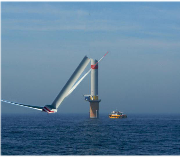
Figure 1.
A wind turbine depends for its power on the flow of the wind energy, i.e. it varies with the 3rd power of the
wind velocity, v. If v ≤ 5 kn (= 2,5 m/sec) the turbines do not produce electricity. (Their
blades may be
rotated to keep the bearings loose, but there is no output. Note: this is an
example of a turbine's consumption of electricity.) At
19 knots they reach their maximum
capacity, i.e. P = 100 MW (or 200, or 300 MW).
In between the power must be interpolated by:
| P = 0,03644 x (v - 5)3 (or 2x, or 3x) | (1) |
as depicted in
Figure 2.
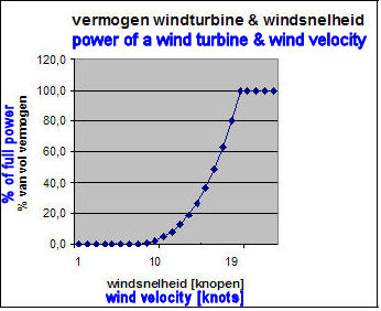
X-axis = wind speed [kn]; Y-axis = % of full power.
This implies a loss that depends on the wind speed. At that site on August 28 this means a varying wind
contribution shown in
Figure 3.
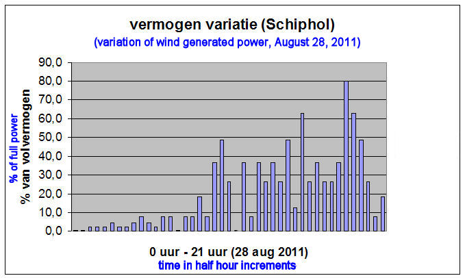
X-axis = time in half hour increments; Y-axis = % of full wind power.
If we would calculate the total power contribution using the old model, on that day the 100 MW wind
project would have saved 4,2% of the use of the conventional gas power plant. (Details of the arithmetic can be found in the Appendix.) Wind
energy experts attribute a 'capacity factor' of 25% to
wind turbines in the Netherlands. That is to say with a name plate capacity of 100 MW the average
contribution over the year would be 25 MW, which means 5% (25/500) saving. However, in 2008 the overall capacity factor
of the wind turbines in the Netherlands was 22,63%16. Thus an
average wind day in 2008 would have saved 4,5%.
We found 4,2% in our example, which means that August 28 was just slightly less than an average wind day that year.
But, because of the cycling effect the real result is appreciably different.
The Schiphol record tells us the wind speed every half hour (i). With (1) we find the wind power, Pw,i, and the power of the adjusting CCGT+, PGT,i.
| PGT,i = 500 - Pw,i | (2) |
We calculate the fuel consumption during that half hour with the quasi stationary method. That is we split the 30
minutes in a part in which the CCGT+ produces stationary and a part at which the system is ramping from the previous level
PGT,i-1 to PGT,i. For the first part we use:
ηi and for the second: 0,5 x (ηi-1+
ηi).
For details see Appendix.
We know what cycling does in the case of 100% - 80% - 100% for a 500 MW generator.
During a full cycle there are three phases: up,
down & stationary. In a cycle during a full hour with 12 MW/min, these last ~8,3 min, ~8,3 min and ~43,4 min.
During the 43,4 min there is saving. During the two times 8,3 min there is saving while going down and
extra fuel consumption going up. The net cycle cost in the example is the same whether it happens during an
hour or during a half hour as long as the ramp rate remains 12 MW/min. Only the stationary minutes are less.
The net cycle costs will depend on the amplitude
of the cycle and to some extend on the power level at which the CCGT operates. Also the duration of cycling
depends on the amplitude.
We assume:
- The net cycle loss does not depend on the power level. (Probably the loss at low power i.e. with high wind penetration increases, because the relative diferences are bigger and the CCGT has a lower efficiency there.)
- The net cycle loss is proportional to the amplitude. It is zero if the amplitude = 0 (stationary) and at amplitude = 100 MW the loss is as in the example.
- During the half hours we only see half cycles. We assume that they require also only half the net loss. Because the wind speed over a longer period always returns to its earlier value, our CCGT ramps as much up as down, which justifies this assumption.
Now we are able to compute for each half hour the savings of the system. (Quasi stationary saving minus the pertaining cycle loss.) Summing them up and comparing them with the fuel use of our CCGT at full power, we obtain the percentage fuel (and emission) saving over the 21˝ hour period.
6. Energy costs of construction and installation.
We use the data of the energy costs for construction and installation of the research department of Volker Wessels Stevin, a major installer of wind turbines5: 1,5 year wind turbine production to recover the needed energy. If we then assume the life time of a wind turbine to be 15 years, it means that 10% of its production must be deducted to compensate for the earlier loss. We shall also do our calculation for a life time of 30 years, meaning a 5% deduction.
7. Energy costs of connection and adaptation to the grid.
Here we'll work with the same deductions as in § 6, see § 4c.
8. Need for more OCGTs.
OCGTs are the best generators to compensate for rapid variations. Their thermal efficiency
is about half of that of a CCGT. OCGTs are always used because of fast changes of demand. Now the variations
of wind power add to the variations of demand, which results in more low
efficiency / high fuel use production.
We assume that with wind projects of 100 MW, resp. 200 MW and 300 MW the participation of OCGTs has to be increased by
resp. 3, 6 and 10%. That we are not dealing here with a negligible complication can be illustrated with
a comic remark by the CEO of the Gas Union, the main natural gas supplier in the Netherlands. While he was being
interviewed on Dutch TV about the huge activity of constructing new gas pipe lines, he said: "It is because all that
wind takes so much gas."
In our computations we reduced the effective η of the conventional plant according to the said percentages
with the η of the OCGTs, for which we took ηOCGt =
0,32.
The other factors mentioned in §§ 4f, 4g & 4h we leave out.
9. Results & conclusions.
The result of our calculations are summarised in table 4. One must keep in mind that the conventional fossil fuel (gas) plant is capable to satisfy the whole electricity demand by itself. So all costs for buying the wind equipment, the costs of installation and those of the extra cables and net adaptation are extra. (See Appendix for the algorithmes.)
Fuel saving and CO2 emission saving through wind projects according to
different models and including other relevant factors.
Results for a 500 MW production provided by a modern gas fired plant with design capacity of 500 MW
together with a wind project with name plate capacity, V, near Schiphol on a normal windy day.
| V | 100 MW wind | 200 MW wind | 300 MW wind |
|---|---|---|---|
| Old model | 4,2% | 8,3% | 12,5% |
| Quasi stationary ≈ current | 3,5% | 7,1% | 10,7% |
| Including 'cycling' | 1,4% | 2,9% | 4,4% |
| Ibid. incl. lifetime 30 yr. | 1,0% | 2,0% | 3,1% |
| Same lifetime 15 yr. | 0,6% | 1,2% | 1,9% |
| Same (30 yr.) + OCGT | -0,3% | -0,5% | -1,0% |
| Same (15 yr.) + OCGT15 | -0,8% | -1,4% | -2,3% |
It is clear. The alleged savings provided by wind projects that could cover 20%, 40% or 60% of the electricity demand during favourable winds are not just negligible, they are even negative, when the most known relevant factors are taken into account. As we remarked before, there is substantial evidence that a life time of 15 year is not an exaggeration. We mentioned the park that had to be renewed after 12 years. That was an onshore development. The projects to be constructed off shore operate under more difficult circumstances. Therefore we conclude:
| NON-SUSTAINABLE.
A 300 MW nameplate wind project near Schiphol on August 28, 2011, a normal windy day, during 21,5 h would have increased the amount of natural gas needed for the electricity production of 500 MW with 47150 m3 gas. This would have caused an extra emission of 117,9 ton CO2 into the atmosphere. |
The wind projects do not fulfill 'sustainable' objectives. They cost more fuel than they save and they cause no CO2 saving, in the contrary they increase our environmental 'foot print'.
A decision to invest Billions (thousands of millions) of Euros in the construction of wind projects 'to save fossil fuel and to reduce CO2 emission' is irresponsible. There are no savings, THERE IS LOSS!
We do not consider it likely that more knowledge of the factors influencing the present outcomes would change our results appreciably. It is more likely that including the factors we identified as not having sufficient data on, would actually increase the loss.
Acknowledgement: John Droz Jr. pointed my attention to flaws in the English language, which I tried to repair as much
as I could.
Nieuwegein, October 7, 2011.
Latest rev.: November 20th.
Referenties & noten.
(The Dutch report tries to explain the subject to the laymen.)
savings of resp. 1,2%; 2,6% and 3,7% for 100 MW wind, 200 MW wind and 300 MW wind,
i.e. 20%, 40% and 60% of the total demand capacity in the form of wind turbines.
These are also absurd
low savings in the view of the economics of electricity production.